vignette("spifa") fits the full spatial model directly,
using a discrimination restriction and a spatial range prior already
decided. In practice both could be informed by previous knowledge or a
preliminary analysis on the data itself. This vignette walks through
that preliminary analysis, then fits the full model:
- Perform non-spatial exploratory item factor analysis to suggest a discrimination structure using the mirt package.
- Analyse the empirical variogram of that fit’s factor scores to suggest a spatial range using the gstat package.
- Fit the full spatial model with
spifa(), using the restriction and range prior from the previous two steps.
#> Loading required package: stats4#> Loading required package: lattice#> Linking to GEOS 3.12.1, GDAL 3.8.4, PROJ 9.4.0; sf_use_s2() is TRUEStep 1: Discrimination structure with mirt
mirt() requires named item columns;
ipixuna$items doesn’t have any, so we name them here:
#>      item1 item2 item3 item4 item5 item6 item7 item8 item9 item10
#> [1,]     0     1     1     0     1     1     1     1     1      1
#> [2,]     1     0     0     1     0     1     1     1     1      0
#> [3,]     1     1     1     1     0     0     0     1     1      1
#> [4,]     0     0     0     0     0     0     0     0     0      0
#> [5,]     1     0     1     0     1     1     1     1     1      1
#> [6,]     0     0     0     0     0     0     0     0     0      0
We fit an exploratory (unrestricted) 2PL item factor model and rotate it (varimax) towards a simple structure:
#> Warning: EM cycles terminated after 500 iterations.
loadings <- summary(efa, rotate = "varimax", verbose = FALSE)$rotF
loadings
#>
#> Loadings:
#> F1 F2 F3
#> item1 0.993
#> item2 0.351 0.438 0.373
#> item3 0.249 0.409 0.654
#> item4 0.741
#> item5 0.967 -0.250
#> item6 0.807 0.150 -0.164
#> item7 0.741 0.115 0.323
#> item8 0.181 0.145 0.750
#> item9 0.589 0.506 0.496
#> item10 0.875 0.241 0.404
#>
#> F1 F2 F3
#> SS loadings 3.471 1.78 2.225Thresholding small loadings to zero turns this into a
0/1 restriction:
A <- (abs(loadings) > 0.24) * 1
A
#> F1 F2 F3
#> item1 0 1 0
#> item2 1 1 1
#> item3 1 1 1
#> item4 0 0 1
#> item5 1 1 0
#> item6 1 0 0
#> item7 1 0 1
#> item8 0 0 1
#> item9 1 1 1
#> item10 1 1 1This is only one approach, different rotations could be applied
depending on the questionnaire and the latent construct under analysis.
In this example, we will use A to constrain discrimination
parameters to zero.
Step 2: Spatial range with gstat
The second thing vignette("spifa") takes as given is
priors$range, the prior for each Gaussian process’s spatial
range. mirt’s factor scores give a first estimate of each
household’s latent abilities, which we can examine spatially with an
empirical variogram.
Estimate the latent factors
First, we obtain the estimated latent factors using
fscores from mirt:
fscore <- fscores(efa, rotate = "varimax")
colnames(fscore) <- paste0("F", seq_len(nfactors))
head(fscore)
#> F1 F2 F3
#> [1,] 1.3211407 -0.08912794 0.40562255
#> [2,] -0.5322310 0.80842440 0.08238761
#> [3,] -0.5511549 1.13429362 1.26588181
#> [4,] -1.1083551 -0.63914342 -0.86797847
#> [5,] 0.9604463 1.01333822 0.05713584
#> [6,] -1.1083551 -0.63914342 -0.86797847Then, we need to geo-reference these factor scores in order to
perform spatial analysis. gstat uses the default
coordinates units to compute distances between locations, so we will
also transform the coordinates system to a planar one where distances
can be computed in meters:
fscore_sf <- st_sf(
  id = ipixuna$id, wealth = ipixuna$wealth, as.data.frame(fscore),
  geometry = st_transform(st_geometry(ipixuna), 32719)
)
fscore_sf
#> Simple feature collection with 100 features and 5 fields
#> Geometry type: POINT
#> Dimension: XY
#> Bounding box: xmin: 201883.2 ymin: 9219014 xmax: 203528.6 ymax: 9221070
#> Projected CRS: WGS 84 / UTM zone 19S
#> First 10 features:
#> id wealth F1 F2 F3 geometry
#> 1 1 -0.57212306 1.32114072 -0.08912794 0.40562255 POINT (202051.7 9219614)
#> 2 2 -0.92003870 -0.53223099 0.80842440 0.08238761 POINT (203142.2 9221070)
#> 3 3 1.23197630 -0.55115490 1.13429362 1.26588181 POINT (203106.4 9220133)
#> 4 4 0.30801774 -1.10835509 -0.63914342 -0.86797847 POINT (202804.6 9220098)
#> 5 5 -0.06247617 0.96044628 1.01333822 0.05713584 POINT (203407.1 9219495)
#> 6 6 2.05414943 -1.10835509 -0.63914342 -0.86797847 POINT (202764.3 9220705)
#> 7 7 2.30552728 -1.42214199 0.88292663 -0.98076254 POINT (202274.5 9219862)
#> 8 8 0.16913811 -0.70539249 0.88627583 -0.01411773 POINT (203219 9220140)
#> 9 9 -0.21989753 0.03337854 -1.44721269 -0.92935929 POINT (202584.1 9219519)
#> 10 10 -0.91744763 0.08478991 1.65515016 0.33080265 POINT (203053.4 9220554)Evaluate predictors effects
We can evaluate the effect of wealth on this estimated latent factors:
fscore_sf |>
  tidyr::pivot_longer(F1:F3) |>
  ggplot(aes(wealth, value)) +
    geom_point() +
    geom_smooth(method = 'lm', formula = y ~ x) +
    facet_wrap(~ name) +
    theme_bw()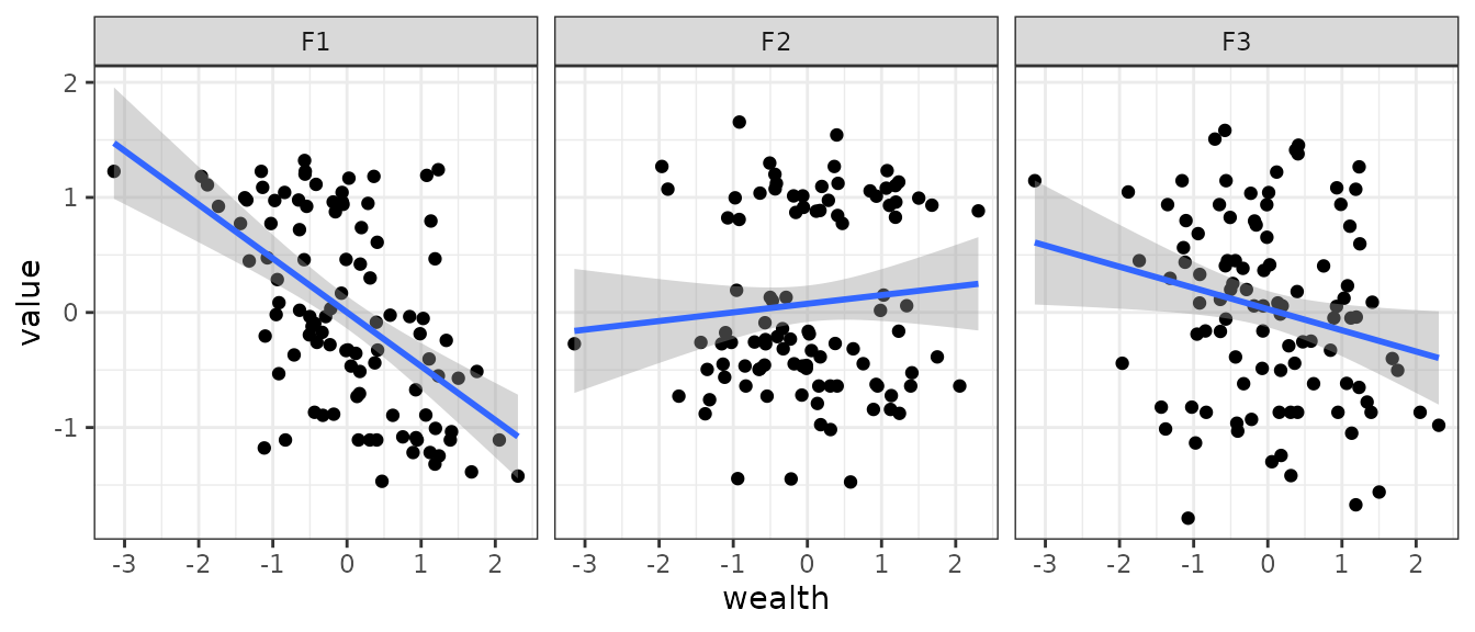
There seems to be an effect in F1 and F3, so we will analyse the
residual spatial structure after taking into account wealth
effect:
Evaluate the spatial structure
From gstat, we can use variogram() to
obtain the empirical variogram, vgm() to define a
theoretical variogram and fit.variogram() to fit the
theoretical model to the empirical variogram.
vg1 <- variogram(F1 ~ wealth, fscore_sf, width = 20, cutoff = 1000)
vg1_fit <- fit.variogram(vg1, model = vgm(psill = 0.6, "Exp", range = 100, nugget = 0.1))
vg1_fit
#> model psill range
#> 1 Nug 0.1864819 0.00000
#> 2 Exp 0.3435766 27.67716
plot(vg1, vg1_fit, pch = 19, main = "F1")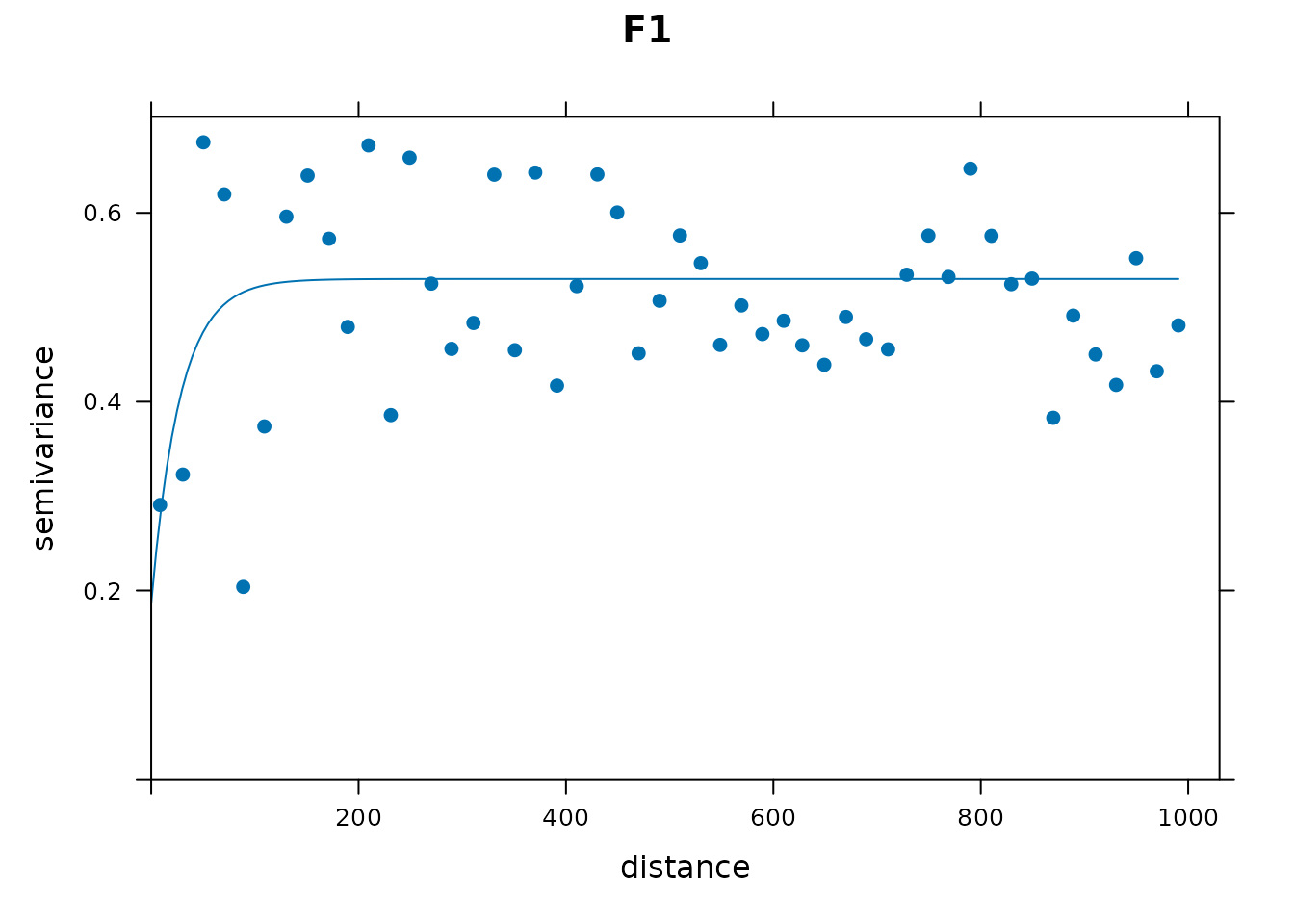
For F1, we can see that there is some evidence of spatial correlation at small scale.
vg2 <- variogram(F2 ~ wealth, fscore_sf, width = 50, cutoff = 1000)
vg2_fit <- fit.variogram(vg2, model = vgm(psill = 0.6, "Exp", range = 100, nugget = 0.1))
vg2_fit
#> model psill range
#> 1 Nug 0.2075966 0.0000
#> 2 Exp 0.4376844 170.9042
plot(vg2, vg2_fit, pch = 19, main = "F2")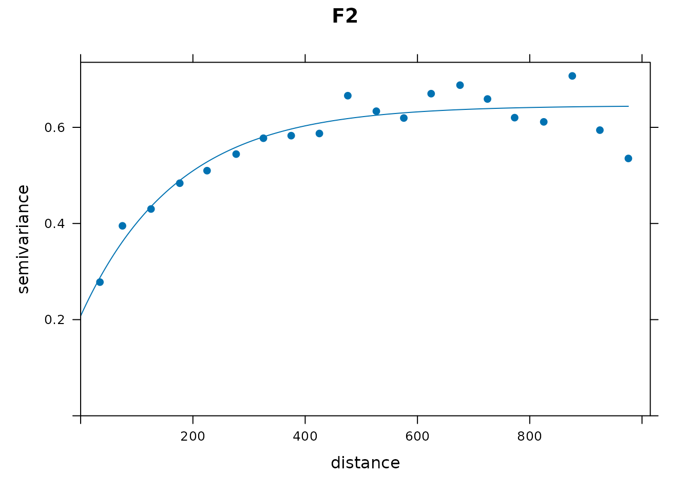
For F2, there is a much clearer spatial structure with a range
parameter around 170.
vg3 <- variogram(F3 ~ wealth, fscore_sf, width = 50, cutoff = 800)
vg3_fit <- fit.variogram(vg3, model = vgm(psill = 0.6, "Exp", range = 100, nugget = 0.1))
#> Warning in fit.variogram(vg3, model = vgm(psill = 0.6, "Exp", range = 100, : No convergence after
#> 200 iterations: try different initial values?
vg3_fit#> model psill range
#> 1 Nug 0.0000000 0.0000
#> 2 Exp 0.6250431 16.9448
plot(vg3, vg3_fit, pch = 19, main = "F3")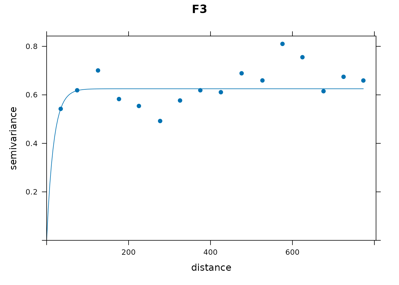
For F3 also the range parameter seems to be small.
In general, there is some evidence of spatial correlation in the
latent factors, and specifically in F2 the spatial structure is strong
with a range parameter around 170. This gives a good understanding of
plausible values for the range parameters of our spifa
model. However, remember that the spifa and
mirt models are not exactly the same, so these values
should be taken only as a reference to decide on our
constraints and priors.
Step 3: Spatial modelling with spifa
With A from Step 1 and a range prior from Step 2 in
hand, spifa() can fit the full spatial model, one
independent Gaussian process per factor by default. For the range prior,
F2’s estimate is the one clear signal – with only 100 households, F1 and
F3’s much smaller ranges are more likely noise than genuine short-range
structure – so we use a common reference value of 150 (close to F2’s
~170) for all three factors:
set.seed(1)
samples <- spifa(
  items ~ wealth, data = ipixuna, nfactors = nfactors,
  burnin = 1000, niter = 4000,
  constraints = list(discrimination = A, loading = diag(nfactors)),
  priors = list(range = list(initial = 150, mean = 150, sd = 0.4)))
samples
#> Item factor analysis model: spifa_pred
#> Formula: items ~ wealth
#> Dimensions: 100 respondents, 10 items, 3 latent factors, 3 spatial processes
#> MCMC: 1 chain, iter = 4000, thin = 1, samples = 4000
#>
#> Item model parameters:
#> mean median sd q10 q90 ess_bulk rhat
#> c[1] -0.498 -0.497 0.33 -0.893 -0.090 76 1
#> c[2] -0.549 -0.551 0.25 -0.850 -0.237 92 1
#> c[3] -0.574 -0.574 0.28 -0.938 -0.219 104 1
#> c[4] -0.352 -0.349 0.21 -0.612 -0.098 198 1
#> c[5] -0.370 -0.350 0.29 -0.747 -0.016 129 1
#> c[6] 0.015 0.019 0.22 -0.263 0.285 236 1
#> c[7] 0.215 0.203 0.23 -0.070 0.516 185 1
#> c[8] 0.159 0.147 0.22 -0.108 0.451 272 1
#> c[9] 0.704 0.661 0.38 0.271 1.193 66 1
#> c[10] 0.391 0.379 0.31 0.011 0.789 158 1
#> A[2,1] -0.313 -0.306 0.22 -0.593 -0.039 238 1
#> A[3,1] -0.106 -0.103 0.23 -0.401 0.180 310 1
#> A[5,1] -1.698 -1.667 0.45 -2.300 -1.135 100 1
#> A[6,1] -1.241 -1.214 0.31 -1.651 -0.859 151 1
#> A[7,1] -1.122 -1.095 0.33 -1.544 -0.723 85 1
#> A[9,1] -1.041 -1.007 0.34 -1.503 -0.628 137 1
#> A[10,1] -1.414 -1.397 0.34 -1.875 -0.989 168 1
#> A[1,2] 1.189 1.153 0.38 0.722 1.715 89 1
#> A[2,2] 0.715 0.705 0.22 0.440 1.008 426 1
#> A[3,2] 0.688 0.680 0.29 0.314 1.074 195 1
#> A[5,2] -0.111 -0.099 0.31 -0.523 0.279 141 1
#> A[9,2] 0.948 0.927 0.38 0.475 1.430 115 1
#> A[10,2] 0.193 0.192 0.31 -0.190 0.577 155 1
#> A[2,3] 0.494 0.484 0.25 0.180 0.816 266 1
#> A[3,3] 0.924 0.920 0.23 0.637 1.217 324 1
#> A[4,3] 0.863 0.833 0.27 0.544 1.238 137 1
#> A[7,3] 0.652 0.630 0.25 0.351 0.984 177 1
#> A[8,3] 1.009 0.986 0.29 0.656 1.401 214 1
#> A[9,3] 0.833 0.819 0.30 0.456 1.229 181 1
#> A[10,3] 1.068 1.042 0.33 0.679 1.503 162 1
#>
#> Factor model parameters:
#> mean median sd q10 q90 ess_bulk rhat
#> B[1,1] 0.3593 0.352 0.11 0.22 0.503 186 1.0
#> B[1,2] 0.0098 0.013 0.10 -0.13 0.142 292 1.0
#> B[1,3] -0.2136 -0.209 0.10 -0.35 -0.084 529 1.0
#> T[1,1] 0.9689 0.962 0.11 0.83 1.134 35 1.0
#> T[2,2] 0.9867 0.970 0.19 0.75 1.256 32 1.0
#> T[3,3] 0.9811 0.965 0.14 0.83 1.155 40 1.0
#> phi[1] 82.1705 80.151 19.87 57.43 106.581 33 1.0
#> phi[2] 172.9428 165.389 55.89 108.35 243.588 45 1.0
#> phi[3] 115.9469 114.255 29.58 82.03 155.454 55 1.0
#> Corr[2,1] -0.1652 -0.255 0.47 -0.76 0.511 38 1.1
#> Corr[3,1] -0.3286 -0.334 0.23 -0.60 -0.073 39 1.1
#> Corr[3,2] -0.3482 -0.429 0.38 -0.81 0.181 46 1.1
#>
#> ess_bulk is the bulk effective sample size; rhat is the potential
#> scale reduction factor on split chains (Rhat = 1 at convergence).
#> Use summary() for the full set of statistics (incl. ess_tail).Note this uses spifa()’s own default (non-informed)
initial values for everything except the spatial range – the same
starting point a real user, without further domain knowledge, would use.
The full analysis can now proceed using the methods presented in
vignette("spifa") and the package’s other vignettes.
Visualize
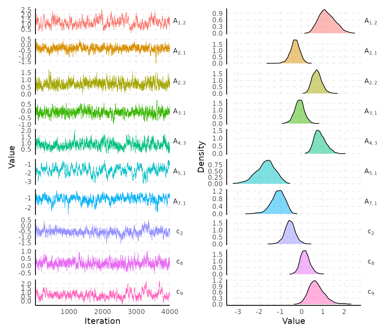
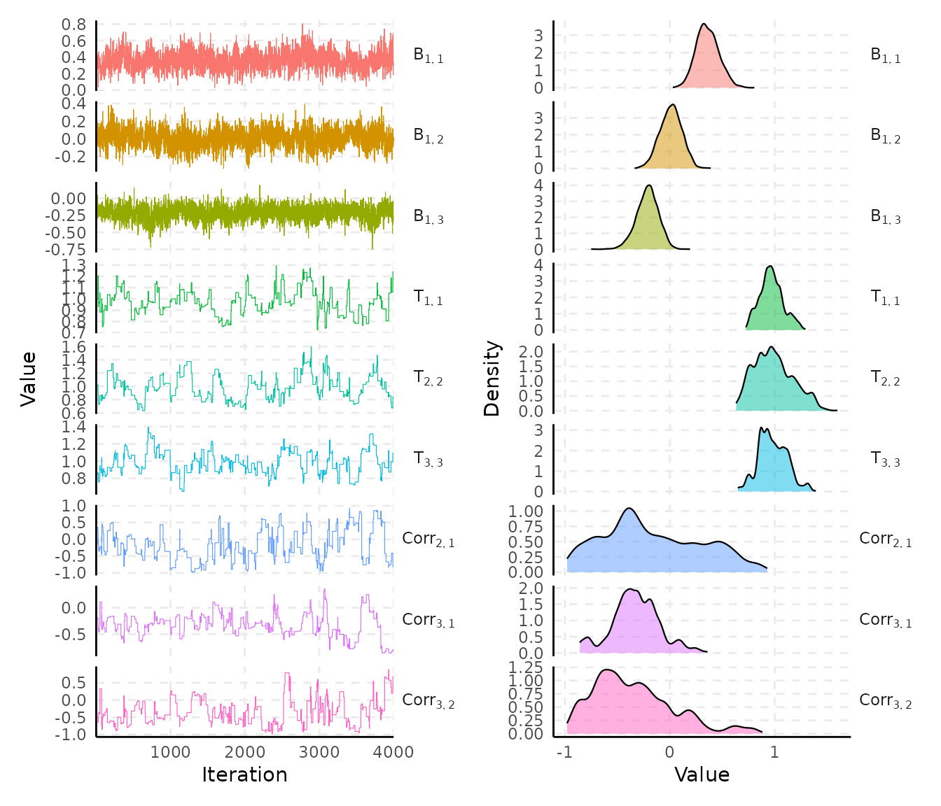
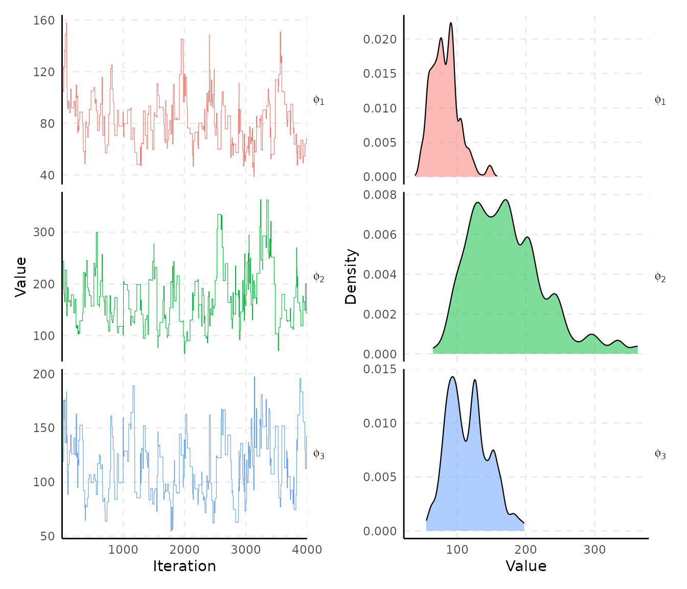
Let’s visualize the chains and densities of the posterior. Observe which parameters have better mixing than others.
Predict
Let’s visualize the spatial pattern of the latent factors mean prediction.
pred_samples <- predict(samples)
plot_predict(pred_samples) +
  scale_colour_distiller(palette = "RdYlBu")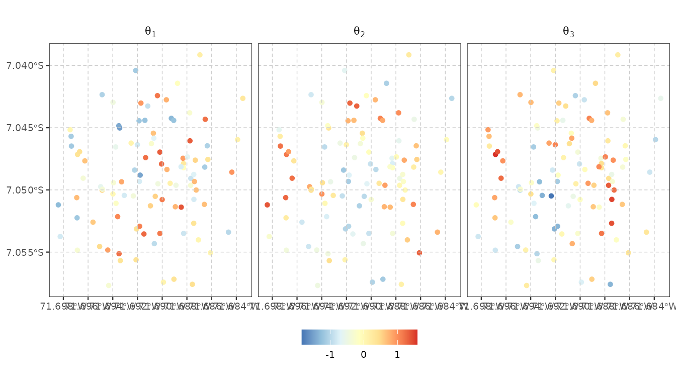
You can continue your analysis using the other methods and functions shown in the package’s vignettes.