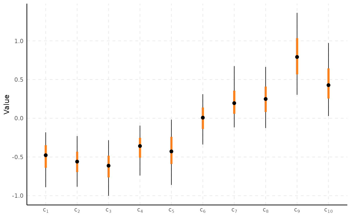
Interval Plot of spifa Posterior Samples — plot

Draws a caterpillar/forest plot of posterior credible intervals directly from a fitted spifa model: one row per parameter, with a thin line for the prob_outer interval, a thick line for the prob interval, and a point at the point_est, computed directly from the raw draws (quantiles/median/mean). 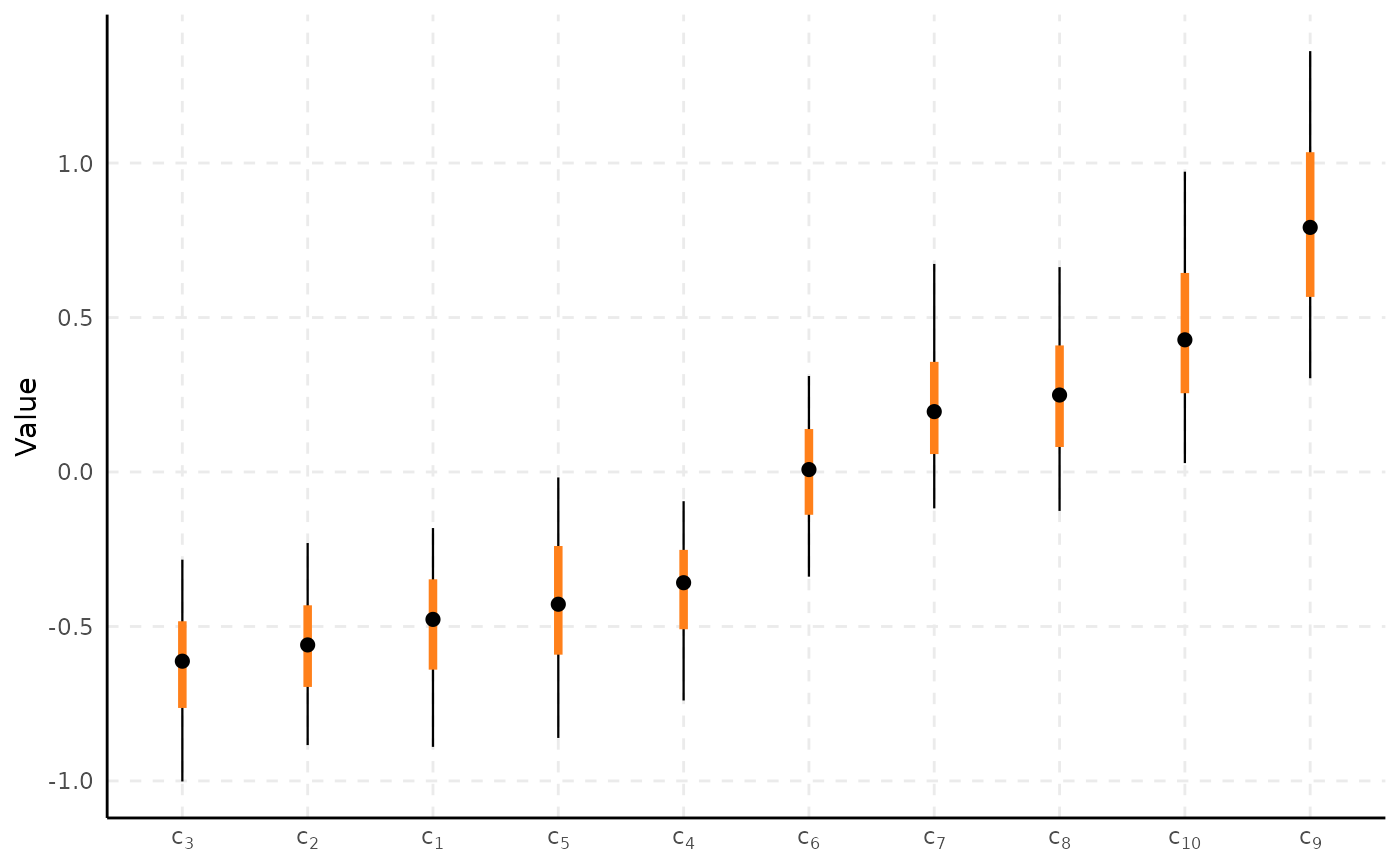Unlike plot_trace/plot_density, this is a single combined view by design – comparing intervals side by side is the whole point, so there is no faceted alternative – but sort can reorder parameters by their point estimate, which a facet can't do usefully across independent panels.

Usage

plot_interval(
  x,
  select,
  horizontal = FALSE,
  burnin = 0,
  thin = 1,
  nshow = NULL,
  prob = 0.5,
  prob_outer = 0.9,
  point_est = c("median", "mean"),
  sort = FALSE,
  reference = NULL,
  ...
)

Arguments

x: A fitted spifa model.
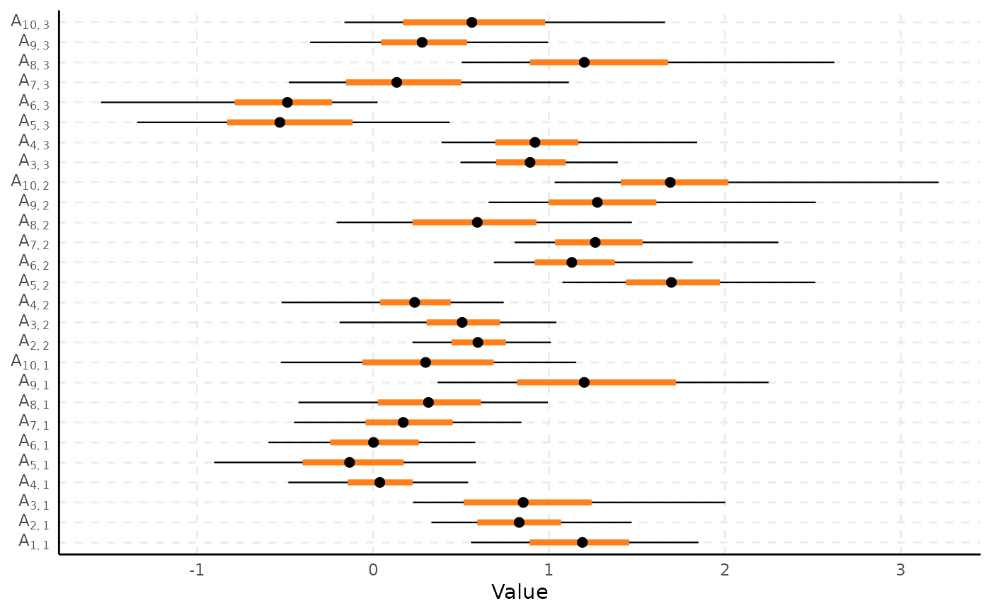
select: Parameters to plot, as in plot_trace.
horizontal: Logical; if FALSE (default), parameters run along the x-axis and values run along the y-axis; if TRUE, the axes are swapped (a forest-plot layout).
burnin: Number of initial iterations to discard.
thin: Thinning interval applied after burnin.
nshow: As in plot_trace (a random subsample when select matches more than nshow parameters), but NULL (show every matched parameter) by default: unlike a faceted plot, a single interval plot stays readable with many more than 10 rows.
prob: Width of the thick (inner) credible interval (a central quantile interval). Defaults to 0.5.
prob_outer: Width of the thin (outer) credible interval. Defaults to 0.9.
point_est: Either "median" (default) or "mean".
sort: Logical; if TRUE, reorder parameters by their point estimate instead of their natural order. Defaults to FALSE.
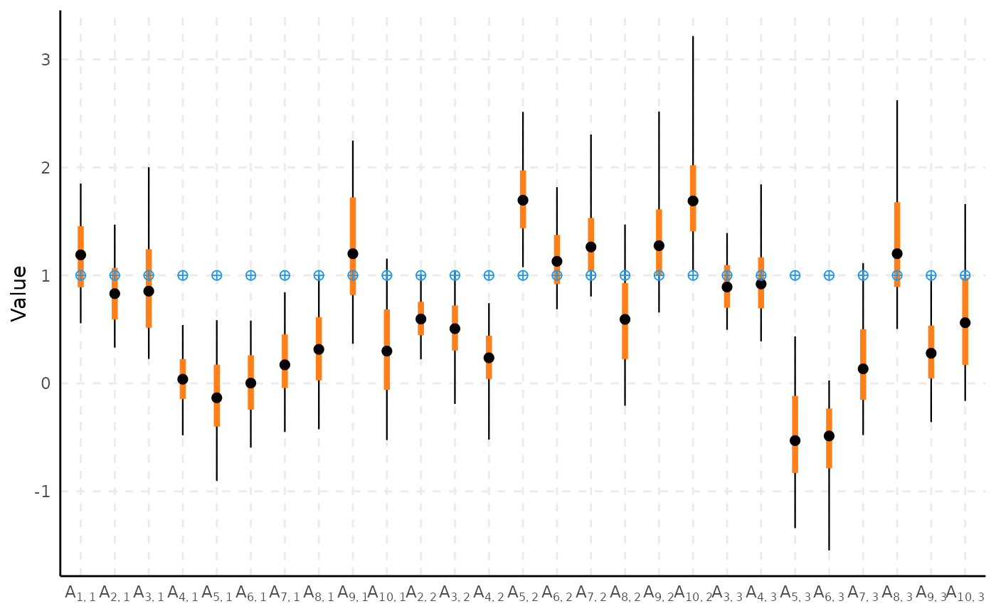
reference: Optional reference values to overlay (e.g. the true values in a simulation study), as a fourth marker alongside the interval and point estimate. Only valid when select is a single group name (e.g. "A"): an unnamed vector or matrix matching that group's own shape (e.g. parameters$discrimination, an nitems x nfactors matrix). Structurally-restricted parameters (dropped internally before plotting) are silently ignored if present in reference.
...: Currently unused.

Value

A ggplot object.

Author

Erick A. Chacón-Montalván

Examples

# \donttest{
data(ipixuna)
samples <- spifa(items ~ 1, data = ipixuna, nfactors = 3, ngp = 0, niter = 1000)

plot_interval(samples, select = "c")

plot_interval(samples, select = "c", sort = TRUE)

plot_interval(samples, select = "A", horizontal = TRUE)


# overlay a reference set of discrimination values (e.g. from theory)
nitems <- ncol(ipixuna$items)
reference_A <- matrix(1, nitems, 3)
plot_interval(samples, select = "A", reference = reference_A)

# }