Bayesian spatial functional clustering

sfclust() is the main user-facing function for Bayesian spatial functional clustering via reversible-jump MCMC. It dispatches on the class of the first argument:

Usage

sfclust(x, ...)

# Default S3 method
sfclust(x, ...)

# S3 method for class 'data.frame'
sfclust(
  x,
  adjacency,
  graphdata = NULL,
  fnames = NULL,
  nclust = 10,
  move_prob = c(0.425, 0.425, 0.1, 0.05),
  logpen = log(1 - 0.5),
  correction = TRUE,
  niter = 100,
  burnin = 0,
  thin = 1,
  nmessage = 10,
  path_save = NULL,
  nsave = nmessage,
  ...
)

# S3 method for class 'stars'
sfclust(
  x,
  nclust = 10,
  graphdata = NULL,
  spnames = NULL,
  move_prob = c(0.425, 0.425, 0.1, 0.05),
  logpen = log(1 - 0.5),
  correction = TRUE,
  niter = 100,
  burnin = 0,
  thin = 1,
  nmessage = 10,
  path_save = NULL,
  nsave = nmessage,
  ...
)

Arguments

x: A data.frame (core interface) or a stars object (stars interface). Dispatch is based on this argument's class. For sfclust.data.frame: a long-format data frame with at least columns id (unique row index) and ids (integer spatial unit index, 1 to ns), plus any response and covariate columns referenced in formula. For sfclust.stars: a stars object containing response variables, covariates, and other necessary data.
...: Additional arguments such as formula, family, and others passed to inla().
adjacency: A square weighted adjacency matrix (ns × ns) encoding spatial contiguity and edge weights. Can be a dense matrix or a sparse Matrix. Typically obtained via igraph::as_adjacency_matrix() on the graph returned by genclust().
graphdata: A list with components graph, mst, and membership as returned by genclust(). If NULL, it is built automatically.
fnames: Character. Name of the column in x that holds the functional index (e.g. "id_time"). Used by plot methods; not required by the algorithm itself. Default is NULL.
nclust: Integer. Initial number of clusters when graphdata = NULL. Ignored if graphdata is provided (default is 10).
move_prob: A numeric vector of probabilities for the MCMC move types: birth, death, change, and hyperparameter (default is c(0.425, 0.425, 0.1, 0.05)).
logpen: A negative numeric value representing the log-scale penalty for increasing the number of clusters by one. The number of clusters is assumed to follow a geometric prior with probability q, making this penalty equal to log(1 - q). For example, if logpen = -50, then a proposal that increases the number of clusters will only be favored if it improves the log marginal likelihood by more than 50.
correction: A logical indicating whether correction to compute the marginal likelihoods should be applied (default is TRUE). This depends on the type of effects included in the INLA model.
niter: An integer specifying the number of MCMC iterations after burn-in (default is 100).
burnin: An integer specifying the number of burn-in iterations to discard (default is 0).
thin: An integer specifying the thinning interval for recording the results (default is 1).
nmessage: An integer specifying how often progress messages should be printed (default is 10).
path_save: A character string specifying the file path to save the results (default is NULL).
nsave: An integer specifying the number of iterations between saved results (default is nmessage).
spnames: Character vector with the names of the spatial dimensions of x. If NULL (default), auto-detected from the stars object dimensions.

Value

An sfclust object (from sfclust.data.frame) or an sfclust_stars object inheriting from sfclust (from sfclust.stars). Both contain:

samples: MCMC trace with membership, log_mlike, and move_counts.
clust: selected clustering with id, membership, and fitted models.

sfclust_stars additionally carries input_args with stars (structural shell of the input), spnames, and fnames, used by spatial plot methods.

Details

sfclust.data.frame(): core interface — takes a pre-built long-format data frame and a weighted adjacency matrix. Use this when working with any data format after converting it yourself.
sfclust.stars(): stars wrapper — takes a stars spatio-temporal object, converts it to long format, builds the spatial graph, and calls the core algorithm.

This implementation draws inspiration from the methods described in the paper: "Bayesian Clustering of Spatial Functional Data with Application to a Human Mobility Study During COVID-19" by Bohai Zhang, Huiyan Sang, Zhao Tang Luo, and Hui Huang, published in The Annals of Applied Statistics, 2023. For further details on the methodology, please refer to:

The paper: doi:10.1214/22-AOAS1643
Supplementary material: doi:10.1214/22-AOAS1643SUPPB

The MCMC algorithm in this implementation is largely based on the supplementary material provided in the paper. However, we have generalized the computation of the marginal likelihood ratio by leveraging INLA (Integrated Nested Laplace Approximation). This generalization enables integration over all parameters and hyperparameters, allowing for inference within a broader family of distribution functions and model terms, thereby extending the scope and flexibility of the original approach. Further details of our approach can be found in our paper "Bayesian spatial functional data clustering: applications in disease surveillance" by Ruiman Zhong, Erick A. Chacón-Montalván, Paula Moraga:

The paper: doi:10.1002/sim.70597

Author

Ruiman Zhong ruiman.zhong@kaust.edu.sa, Erick A. Chacón-Montalván erick.chaconmontalvan@wur.nl, Paula Moraga paula.moraga@kaust.edu.sa

Examples


# \donttest{
if (requireNamespace("INLA", quietly = TRUE)) {
library(sfclust)

# Stars interface: Gaussian model
data(stgaus)
result <- sfclust(stgaus, formula = y ~ f(id_time, model = "rw1"),
  niter = 10, nmessage = 1)

print(result)
summary(result, sort = TRUE)
fitted(result, sort = TRUE)

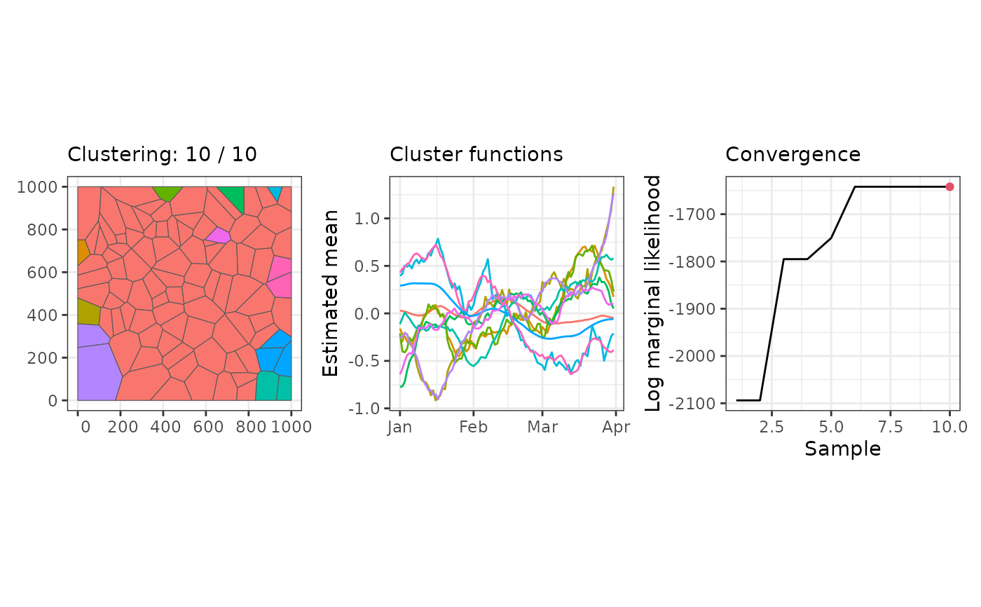
plot(result)
plot_clusters_series(result, var = y)

result2 <- update(result, niter = 2, nmessage = 1)
plot(result2)

# Stars interface: Binomial model
data(stbinom)
result <- sfclust(stbinom, formula = cases ~ poly(id_time, 2) + f(id),
  family = "binomial", Ntrials = population, niter = 10, nmessage = 1)

print(result)
summary(result, sort = TRUE)
fitted(result, sort = TRUE)

plot(result)
plot_clusters_series(result, var = cases/population)

result2 <- update(result, niter = 2, nmessage = 1)
plot(result2)

# data.frame interface: Poisson model
 ns <- 6L; nt <- 4L
 set.seed(4)
 df  <- data.frame(
   id       = seq_len(ns * nt),
   ids      = rep(seq_len(ns), nt),
   id_time  = rep(seq_len(nt), each = ns),
   expected = rep(10L, ns * nt)
 )
 df <- transform(df,
   y = rpois(ns * nt, expected * exp(0.5 * id_time * rep(c(-1, 1), each = ns / 2, nt)))
 )
 adj <- Matrix::sparseMatrix(
   i = c(1, 2, 4, 5, 1, 2, 3), j = c(2, 3, 5, 6, 4, 5, 6),
   x = 1L, dims = c(ns, ns), symmetric = TRUE
 )

 result <- sfclust(df, adjacency = adj, nclust = 3, fnames = "id_time",
   formula = y ~ 1 + id_time, family = "poisson", E = expected,
   niter = 3, burnin = 0, thin = 1, nmessage = 1)

 print(result)
 summary(result, sort = TRUE)
 fitted(result, sort = TRUE)

 plot(result)
 plot_clusters_series(result, var = y)

 result2 <- update(result, niter = 2, nmessage = 1)
 plot(result2)
}
#> Iteration 1: clusters = 11, births = 1, deaths = 0, changes = 0, hypers = 0, log_mlike = -1966.74075178298
#> Iteration 2: clusters = 11, births = 1, deaths = 0, changes = 0, hypers = 0, log_mlike = -1966.74075178298
#> Iteration 3: clusters = 12, births = 2, deaths = 0, changes = 0, hypers = 0, log_mlike = -1871.05703243364
#> Iteration 4: clusters = 12, births = 2, deaths = 0, changes = 0, hypers = 0, log_mlike = -1871.05703243364
#> Iteration 5: clusters = 12, births = 2, deaths = 0, changes = 0, hypers = 0, log_mlike = -1871.05703243364
#> Iteration 6: clusters = 13, births = 3, deaths = 0, changes = 0, hypers = 0, log_mlike = -1815.85190290124
#> Iteration 7: clusters = 13, births = 3, deaths = 0, changes = 0, hypers = 0, log_mlike = -1815.85190290124
#> Iteration 8: clusters = 13, births = 3, deaths = 0, changes = 0, hypers = 0, log_mlike = -1815.85190290124
#> Iteration 9: clusters = 13, births = 3, deaths = 0, changes = 0, hypers = 0, log_mlike = -1815.85190290124
#> Iteration 10: clusters = 14, births = 4, deaths = 0, changes = 0, hypers = 0, log_mlike = -1747.1511074592
#> Within-cluster formula:
#> y ~ f(id_time, model = "rw1")
#> 
#> Clustering hyperparameters:
#>   log(1-q)      birth      death     change      hyper 
#> -0.6931472  0.4250000  0.4250000  0.1000000  0.0500000 
#> 
#> Clustering movement counts:
#>  births  deaths changes  hypers 
#>       4       0       0       0 
#> 
#> Log marginal likelihood (sample 10 out of 10): -1747.151
#> Summary for clustering sample 10 out of 10 
#> 
#> Within-cluster formula:
#> y ~ f(id_time, model = "rw1")
#> 
#> Counts per cluster:
#>  1  2  3  4  5  6  7  8  9 10 11 12 13 14 
#> 71  9  5  4  2  1  1  1  1  1  1  1  1  1 
#> 
#> Log marginal likelihood:  -1747.151 
#> Iteration 1: clusters = 14, births = 0, deaths = 0, changes = 0, hypers = 0, log_mlike = -1747.15108206478
#> Iteration 2: clusters = 15, births = 1, deaths = 0, changes = 0, hypers = 0, log_mlike = -1661.30401229972
#> Warning: Log marginal-likelihood correction not required.
#> Iteration 1: clusters = 11, births = 1, deaths = 0, changes = 0, hypers = 0, log_mlike = -76867.9522131785
#> Iteration 2: clusters = 10, births = 1, deaths = 1, changes = 0, hypers = 0, log_mlike = -76848.8909590969
#> Iteration 3: clusters = 10, births = 1, deaths = 1, changes = 0, hypers = 0, log_mlike = -76848.8909590969
#> Iteration 4: clusters = 11, births = 2, deaths = 1, changes = 0, hypers = 0, log_mlike = -76666.8948761572
#> Iteration 5: clusters = 11, births = 2, deaths = 1, changes = 0, hypers = 0, log_mlike = -76666.8948761572
#> Iteration 6: clusters = 11, births = 2, deaths = 1, changes = 0, hypers = 0, log_mlike = -76666.8948761572
#> Iteration 7: clusters = 11, births = 2, deaths = 1, changes = 1, hypers = 0, log_mlike = -76541.0413121394
#> Iteration 8: clusters = 11, births = 2, deaths = 1, changes = 1, hypers = 0, log_mlike = -76541.0413121394
#> Iteration 9: clusters = 11, births = 2, deaths = 1, changes = 2, hypers = 0, log_mlike = -76452.1427840495
#> Iteration 10: clusters = 11, births = 2, deaths = 1, changes = 2, hypers = 0, log_mlike = -76452.1427840495
#> Within-cluster formula:
#> cases ~ poly(id_time, 2) + f(id)
#> 
#> Clustering hyperparameters:
#>   log(1-q)      birth      death     change      hyper 
#> -0.6931472  0.4250000  0.4250000  0.1000000  0.0500000 
#> 
#> Clustering movement counts:
#>  births  deaths changes  hypers 
#>       2       1       2       0 
#> 
#> Log marginal likelihood (sample 10 out of 10): -76452.14
#> Summary for clustering sample 10 out of 10 
#> 
#> Within-cluster formula:
#> cases ~ poly(id_time, 2) + f(id)
#> 
#> Counts per cluster:
#>  1  2  3  4  5  6  7  8  9 10 11 
#> 52 32  4  4  2  1  1  1  1  1  1 
#> 
#> Log marginal likelihood:  -76452.14 
#> Iteration 1: clusters = 11, births = 0, deaths = 0, changes = 0, hypers = 0, log_mlike = -76452.1431466997
#> Iteration 2: clusters = 11, births = 0, deaths = 0, changes = 0, hypers = 0, log_mlike = -76452.1431466997
#> Warning: Log marginal-likelihood correction not required.
#> Iteration 1: clusters = 3, births = 0, deaths = 0, changes = 0, hypers = 0, log_mlike = -247.318700532878
#> Iteration 2: clusters = 3, births = 0, deaths = 0, changes = 0, hypers = 0, log_mlike = -247.318700532878
#> Iteration 3: clusters = 4, births = 1, deaths = 0, changes = 0, hypers = 0, log_mlike = -84.3225017550345
#> Within-cluster formula:
#> y ~ 1 + id_time
#> 
#> Clustering hyperparameters:
#>   log(1-q)      birth      death     change      hyper 
#> -0.6931472  0.4250000  0.4250000  0.1000000  0.0500000 
#> 
#> Clustering movement counts:
#>  births  deaths changes  hypers 
#>       1       0       0       0 
#> 
#> Log marginal likelihood (sample 3 out of 3): -84.3225
#> Summary for clustering sample 3 out of 3 
#> 
#> Within-cluster formula:
#> y ~ 1 + id_time
#> 
#> Counts per cluster:
#> 1 2 3 4 
#> 2 2 1 1 
#> 
#> Log marginal likelihood:  -84.3225 
#> Iteration 1: clusters = 4, births = 0, deaths = 0, changes = 0, hypers = 0, log_mlike = -84.3225017550345
#> Iteration 2: clusters = 3, births = 0, deaths = 1, changes = 0, hypers = 0, log_mlike = -77.1494805389547

# }