Introduction to sfclust

In this vignette, we demonstrate the basic use of sfclust for spatial functional clustering. Specifically, we focus on a synthetic dataset of disease cases to identify regions with similar disease risk over time.

Packages

We begin by loading the required packages. In particular, we load the stars package as our sfclust package works with spatio-temporal stars objects.

library(sfclust)
library(stars)
library(ggplot2)

Data

The simulated dataset used in this vignette, stbinom, is included in our package. It is a stars object with two variables, cases and population, and two dimensions, geometry and time. The dataset represents the number of cases in 100 regions, observed daily over 91 days, starting in January 2024.

stbinom

#> stars object with 2 dimensions and 2 attributes
#> attribute(s):
#>              Min. 1st Qu.  Median     Mean 3rd Qu.  Max.
#> cases        4632  9295.0 11760.5 11903.97 14238.0 26861
#> population  10911 18733.5 24255.0 23814.57 27517.5 44829
#> dimension(s):
#>          from  to     offset  delta refsys point
#> geometry    1 100         NA     NA     NA FALSE
#> time        1  91 2024-01-01 1 days   Date FALSE
#>                                                                 values
#> geometry POLYGON ((59.5033 683.285...,...,POLYGON ((942.7562 116.89...
#> time                                                              NULL

We can easily visualize the spatio-temporal risk using ggplot and stars::geom_stars. It shows some neighboring regions with similar risk patterns over time.

ggplot() +
    geom_stars(aes(fill = cases/population), data = stbinom) +
    facet_wrap(~ time) +
    scale_fill_distiller(palette = "RdBu") +
    labs(title = "Daily risk", fill = "Risk") +
    theme_bw(base_size = 7) +
    theme(legend.position = "bottom")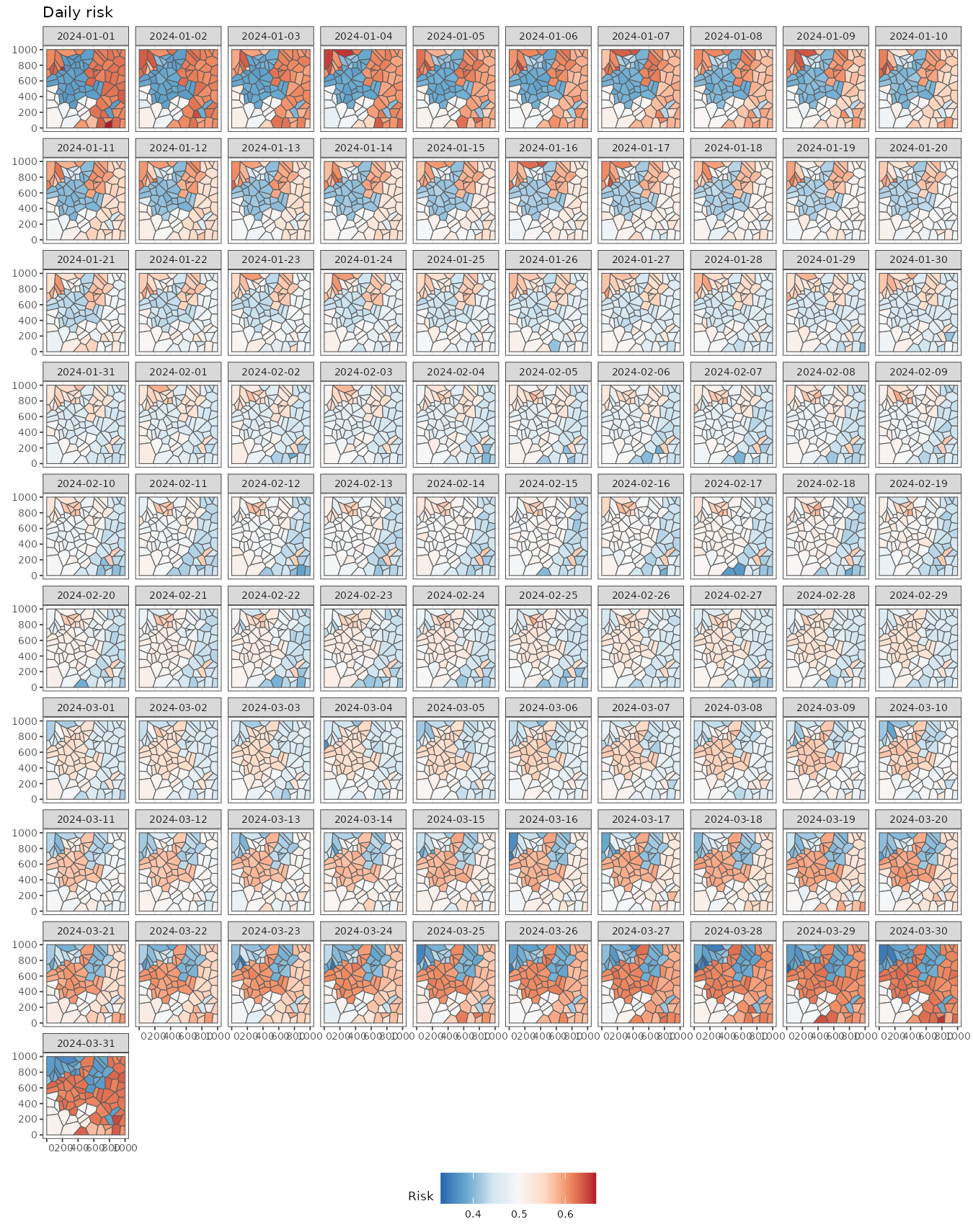

We can aggregate the data for easier visualization using the stars::aggregate function. The following figure displays the weekly mean risk, providing initial insights. For example, the northwestern regions show a higher risk at the beginning (2024-01-01), followed by a decline by the end of the study period (2024-03-25). In contrast, a group of regions on the eastern side exhibits high risk at both the beginning (2024-01-01) and the end (2024-03-25) but lower values in the middle of the study period (2024-02-12).

stweekly <- aggregate(stbinom, by = "week", FUN = mean)
ggplot() +
  geom_stars(aes(fill = cases/population), stweekly) +
  facet_wrap(~ time, nrow = 2) +
  scale_fill_distiller(palette = "RdBu") +
  theme_bw(base_size = 10) +
  theme(legend.position = c(0.93, 0.22))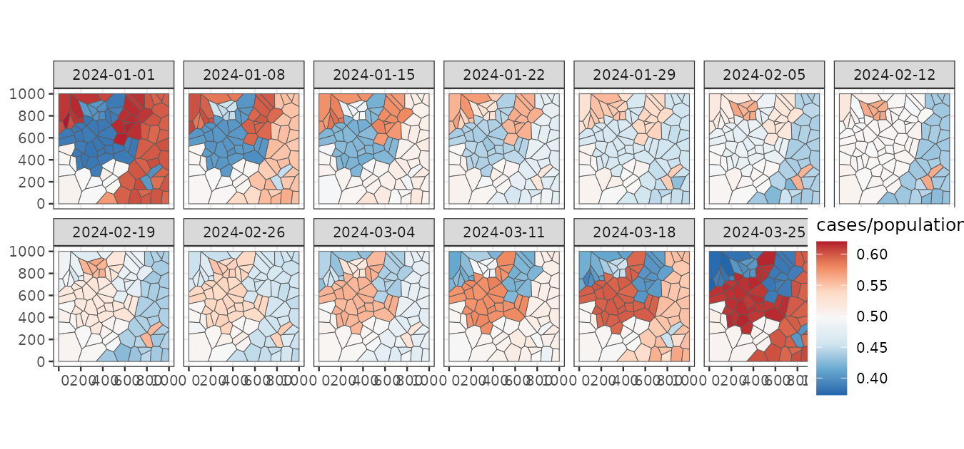

It is also useful to examine trends for each region. This can be done by converting the stars object into a data frame using the as.data.frame function. The visualization reveals that some regions exhibit very similar trends over time. Our goal is to cluster these regions while considering spatial contiguity.

stbinom |>
  st_set_dimensions("geometry", values = 1:nrow(stbinom)) |>
  as.data.frame() |>
  ggplot() +
    geom_line(aes(time, cases/population, group = geometry), linewidth = 0.3) +
    theme_bw() +
    labs(title = "Risk per region", y = "Risk", x = "Time")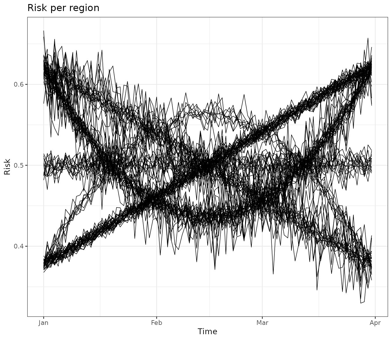

Our methods convert the stars object into a data.frame with custom unique identifiers for the locations and functional dimensions using the data_all. In the following chunk you can see the converted data frame containing, in addition to the original data, a unique identifier for each observation (id), a spatial identifier (ids), and a temporal identifier (id_time).

head(data_all(stbinom))

#>   id ids id_time       time cases population
#> 1  1   1       1 2024-01-01 10023      26062
#> 2  2   2       1 2024-01-01 16022      26411
#> 3  3   3       1 2024-01-01 10829      21504
#> 4  4   4       1 2024-01-01  9358      15325
#> 5  5   5       1 2024-01-01 11702      23981
#> 6  6   6       1 2024-01-01  6914      13807

Clustering

Model

Our model-based approach to spatial clustering requires defining a within-cluster model, where regions within the same cluster share common parameters and latent functions. In this example, given the clustering or partition $M$ , we assume that the observed number of cases ( $y_{it}$ ) for region $i$ at time $t$ is a realization of a Binomial random variable $Y_{it}$ with size $N_{it}$ and success probability $p_{it}$ : $Y_{it} \mid p_{it}, N_{it}, M \stackrel{ind}{\sim} \text{Binomial}(N_{it}, p_{it}).$

Based on our exploratory analysis, the success probability $p_{it}$ is modeled as: $\text{logit}(p_{it}) = \alpha_{c_i} + \boldsymbol{x}_{t}^T\boldsymbol{\beta}_{c_i} + f_{it},$ where $\alpha_{c_i}$ is the intercept for cluster $c_i$ , and $\boldsymbol{x}_{t}$ represents a set of polynomial functions of time that capture global trends with a cluster-specific effect $\boldsymbol{\beta}_{c_i}$ . Additionally, we include an independent random effect, $f_{it} \stackrel{iid}{\sim} \text{Normal}(0, \sigma_{c_i})$ , to account for extra space-time variability.

Since we perform Bayesian inference, we impose prior distributions on the model parameters. The intercept $\alpha_{c_i}$ and regression coefficients $\boldsymbol{\beta}_{c_i}$ follow a Normal distribution, while the prior for the hyperparameter $\sigma_{c_i}$ is defined as: $\log(1/\sigma_{c_i}) \sim \text{LogGamma}(1, 10^{-5}).$ Notably, all regions within the same cluster share the same parameters: $\alpha_{c_i}$ , regression coefficients $\boldsymbol{\beta}_{c_i}$ , and random-effect standard deviation $\sigma_{c_i}$ .

Sampling with `sfclust`

In order to perform Bayesian spatial functional clustering with the model above we use the main function sfclust. The main arguments of this function are:

x: The spatio-temporal data which should be a stars object.
nclust: The initial number of clusters.
spnames: Names of the spatial dimensions (auto-detected if not provided; typically "geometry" for vector data, or c("x", "y") for raster data).
fnames: Names of the functional dimensions. This is a parameter of the data.frame interface only; for the stars interface it is derived automatically as all dimensions other than spnames (e.g. "time") and is not user-settable.
niter: Number of iteration for the Markov chain Monte Carlo algorithm.

Notice that given that sfclust uses MCMC and INLA to perform Bayesian inference, it accepts any argument of the INLA::inla function. Some main arguments are:

formula: expression to define the model with fixed and random effects. sfclust pre-processes the data and creates identifiers for regions ids, functional indices id_<dimname> (e.g. id_time) and space-time id. You can include these identifiers in your formula.
family: distribution of the response variable.
Ntrials: Number of trials in case of a Binomial response.
E: Expected number of cases for a Poisson response.

The following code performs the Bayesian functional clustering for the model explained above with 2000 iterations.

set.seed(7)
result <- sfclust(stbinom, formula = cases ~ poly(time, 2) + f(id),
  family = "binomial", Ntrials = population, niter = 2000)
names(result)

#> [1] "samples" "clust"

The returned object is of class sfclust, which is a list of two elements:

samples: list containing the membership samples, the logarithm of the marginal likelihood log_mlike and the clustering movements move_counts done in total.
clust: list containing the selected membership from samples. This includes the id of selected sample, the selected membership and the models associated to each cluster.

Basic methods

Print

By default, the sfclust object prints the within-cluster model, the clustering hyperparameters, the movement counts, and the current log marginal likelihood.

result

#> Within-cluster formula:
#> cases ~ poly(time, 2) + f(id)
#> 
#> Clustering hyperparameters:
#>   log(1-q)      birth      death     change      hyper 
#> -0.6931472  0.4250000  0.4250000  0.1000000  0.0500000 
#> 
#> Clustering movement counts:
#>  births  deaths changes  hypers 
#>      58      58      21      98 
#> 
#> Log marginal likelihood (sample 2000 out of 2000): -61286.27

The output indicates that the within-cluster model is specified using the formula cases ~ poly(time, 2) + f(id), which is compatible with INLA. This formula includes polynomial fixed effects and an independent random effect per observation.

The displayed hyperparameters are used in the clustering algorithm. The hyperparameter log(1-q) = -0.693 penalizes the increase of clusters, while the other parameters control the probabilities of different clustering movements:

The probability of splitting a cluster is 0.425.
The probability of merging two clusters is 0.425.
The probability of simultaneously splitting and merging two clusters is 0.1.
The probability of modifying the minimum spanning tree is 0.05.

Users can modify these hyperparameters as needed. The output also displays clustering movements. The output summary indicates the following:

Clusters were split 58 times.
Clusters were merged 58 times.
Clusters were simultaneously split and merged 21 times.
The minimum spanning tree was updated 98 times.

Finally, the log marginal likelihood for the last iteration (2000) is reported as -61,286.27.

Plot

The plot method generates three main graphs:

A map of the regions colored by clusters.
The mean function per cluster.
The log marginal likelihood for each iteration.

In our example, the left panel displays the regions grouped into the 10 clusters found in the 2000th (final) iteration. The middle panel shows the mean linear predictor curves for each cluster. Some clusters exhibit linear trends, while others follow quadratic trends. Although some clusters have similar mean trends, they are classified separately due to differences in other parameters, such as the variance of the random effects.

Finally, the right panel presents the log marginal likelihood for each iteration. The values stabilize around iteration 1500, indicating that any clustering beyond this point can be considered a reasonable realization of the clustering distribution.

plot(result, sort = TRUE, legend = TRUE)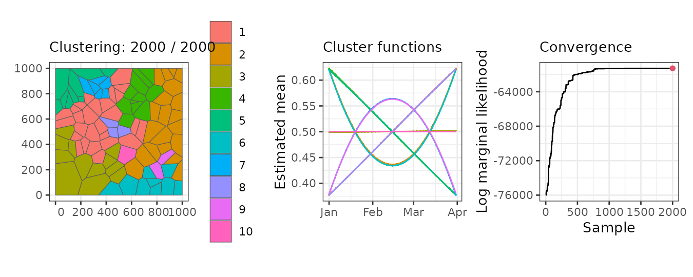

Summary

Once convergence is observed in the clustering algorithm, we can summarize the results. By default, the summary is based on the last sample. The output of the summary method confirms that it corresponds to the 2000th sample out of a total of 2000. It also displays the model formula, similar to the print method.

Additionally, the summary provides the number of members in each cluster. For example, in this case, Cluster 1 has 27 members, Cluster 2 has 12 members, and so on. Finally, it reports the associated log marginal likelihood.

summary(result)

#> Summary for clustering sample 2000 out of 2000 
#> 
#> Within-cluster formula:
#> cases ~ poly(time, 2) + f(id)
#> 
#> Counts per cluster:
#>  1  2  3  4  5  6  7  8  9 10 
#> 27 12  9 11  9  2  6 20  1  3 
#> 
#> Log marginal likelihood:  -61286.27

We can also summarize any other sample, such as an earlier iteration. The output clearly indicates that the log marginal likelihood is typically smaller in earlier samples. Keep in mind that all other sfclust methods use the last sample by default, but you can specify a different sample if needed.

summary(result, sample = 500)

#> Summary for clustering sample 500 out of 2000 
#> 
#> Within-cluster formula:
#> cases ~ poly(time, 2) + f(id)
#> 
#> Counts per cluster:
#>  1  2  3  4  5  6  7  8  9 10 11 12 13 14 15 16 17 18 19 20 21 22 23 24 25 
#> 24  3  6  8  4  1  1  1  3 17  1  2  8  1  1  6  1  1  2  3  1  1  1  1  2 
#> 
#> Log marginal likelihood:  -61992.2

Cluster labels are assigned arbitrarily, but they can be relabeled based on the number of members using the option sort = TRUE. The following output shows that, in the last sample, the first seven clusters have more than four members, while the last three clusters have fewer than four members.

summary(result, sort = TRUE)

#> Summary for clustering sample 2000 out of 2000 
#> 
#> Within-cluster formula:
#> cases ~ poly(time, 2) + f(id)
#> 
#> Counts per cluster:
#>  1  2  3  4  5  6  7  8  9 10 
#> 27 20 12 11  9  9  6  3  2  1 
#> 
#> Log marginal likelihood:  -61286.27

Fitted values

We can obtain the estimated values for our model using the fitted function, which returns a stars object in the same format as the original data. It provides the mean, standard deviation, quantiles, and other summary statistics.

pred <- fitted(result)
pred

#> stars object with 2 dimensions and 11 attributes
#> attribute(s):
#>                            Min.       1st Qu.        Median          Mean
#> id                    1.0000000  2275.7500000  4.550500e+03  4.550500e+03
#> ids                   1.0000000    25.7500000  5.050000e+01  5.050000e+01
#> id_time               1.0000000    23.0000000  4.600000e+01  4.600000e+01
#> cases              4632.0000000  9295.0000000  1.176050e+04  1.190397e+04
#> population        10911.0000000 18733.5000000  2.425500e+04  2.381457e+04
#> sid                   1.0000000    25.7500000  5.050000e+01  5.050000e+01
#> mean                 -0.7055729    -0.1988638 -5.554312e-03 -4.677087e-04
#> mean_inv              0.3305778     0.4504473  4.986114e-01  4.998542e-01
#> cluster               1.0000000     1.0000000  4.000000e+00  4.200000e+00
#> mean_cluster         -0.5011533    -0.1986104  1.814918e-04 -4.677297e-04
#> mean_cluster_inv      0.3772697     0.4505100  5.000454e-01  4.998534e-01
#>                        3rd Qu.         Max.
#> id                6.825250e+03 9.100000e+03
#> ids               7.525000e+01 1.000000e+02
#> id_time           6.900000e+01 9.100000e+01
#> cases             1.423800e+04 2.686100e+04
#> population        2.751750e+04 4.482900e+04
#> sid               7.525000e+01 1.000000e+02
#> mean              1.850752e-01 6.887139e-01
#> mean_inv          5.461372e-01 6.656808e-01
#> cluster           7.000000e+00 1.000000e+01
#> mean_cluster      1.898616e-01 5.015424e-01
#> mean_cluster_inv  5.473233e-01 6.228217e-01
#> dimension(s):
#>          from  to     offset  delta refsys point
#> geometry    1 100         NA     NA     NA FALSE
#> time        1  91 2024-01-01 1 days   Date FALSE
#>                                                                 values
#> geometry POLYGON ((59.5033 683.285...,...,POLYGON ((942.7562 116.89...
#> time                                                              NULL

We can easily visualize these fitted values. Note that there are still differences between regions within the same cluster due to the presence of random effects at the individual level.

ggplot() +
    geom_stars(aes(fill = mean_inv), data = pred) +
    facet_wrap(~ time) +
    scale_fill_distiller(palette = "RdBu") +
    labs(title = "Daily risk", fill = "Risk") +
    theme_bw(base_size = 7) +
    theme(legend.position = "bottom")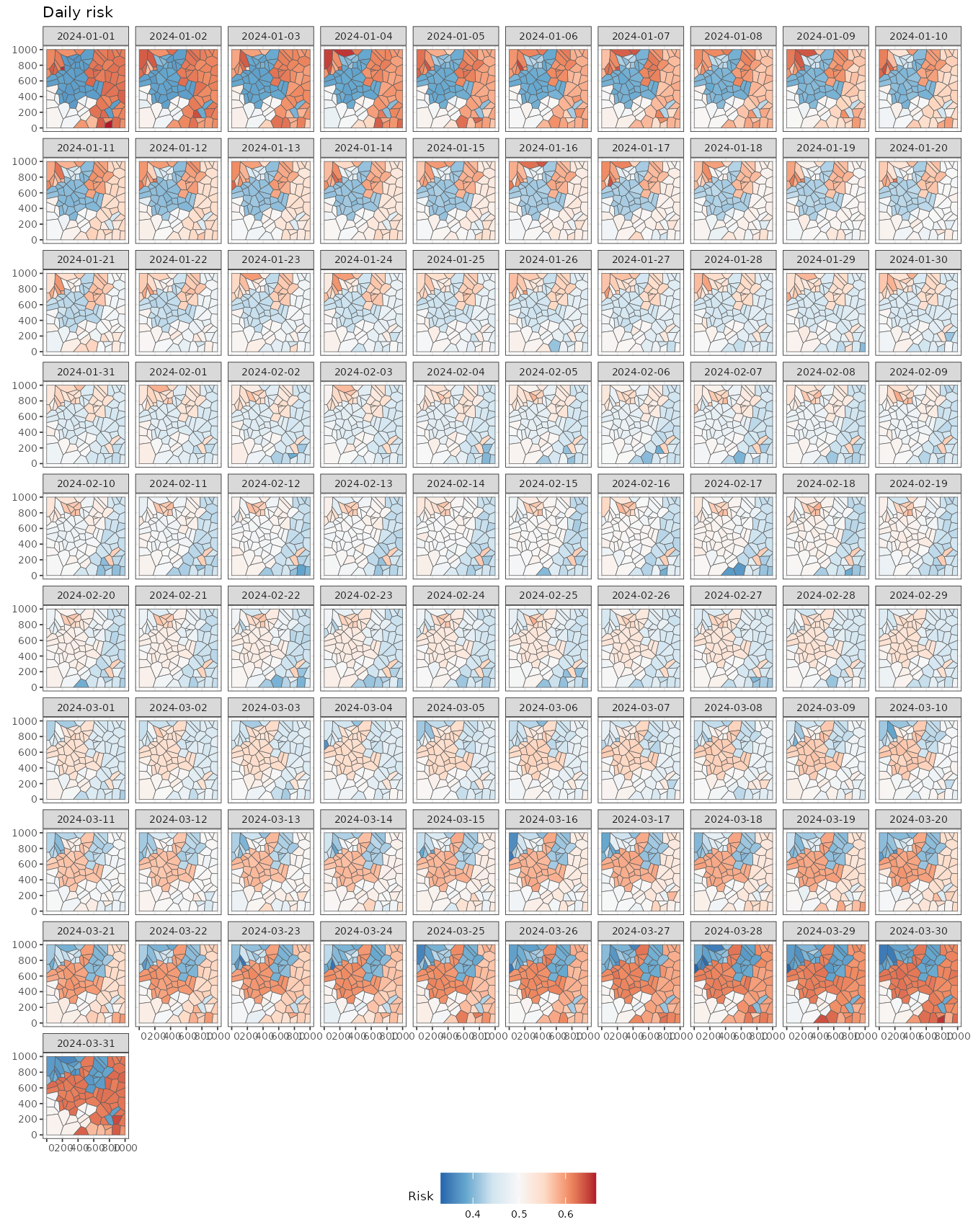

To gain further insights, we can compute the mean fitted values per cluster using aggregate = TRUE. This returns a stars object with cluster-level geometries.

pred <- fitted(result, sort = TRUE, aggregate = TRUE)
pred

#> stars object with 2 dimensions and 2 attributes
#> attribute(s):
#>                         Min.    1st Qu.      Median         Mean   3rd Qu.
#> mean_cluster      -0.5011527 -0.1716051 0.001578615 -0.000589982 0.1701283
#> mean_cluster_inv   0.3772698  0.4572037 0.500394654  0.499856282 0.5424298
#>                        Max.
#> mean_cluster      0.5015421
#> mean_cluster_inv  0.6228217
#> dimension(s):
#>          from to     offset  delta refsys point
#> geometry    1 10         NA     NA     NA FALSE
#> time        1 91 2024-01-01 1 days   Date FALSE
#>                                                                 values
#> geometry POLYGON ((149.5651 508.30...,...,POLYGON ((491.7737 272.18...
#> time                                                              NULL

Using these estimates, we can visualize the cluster-level mean risk evolution over time.

predweekly <- aggregate(pred, by = "week", FUN = mean)
ggplot() +
  geom_stars(aes(fill = mean_cluster_inv), data = predweekly) +
  facet_wrap(~ time, nrow = 2) +
  scale_fill_distiller(palette = "RdBu") +
  labs(fill = "Risk") +
  theme_bw(base_size = 10) +
  theme(legend.position = "bottom")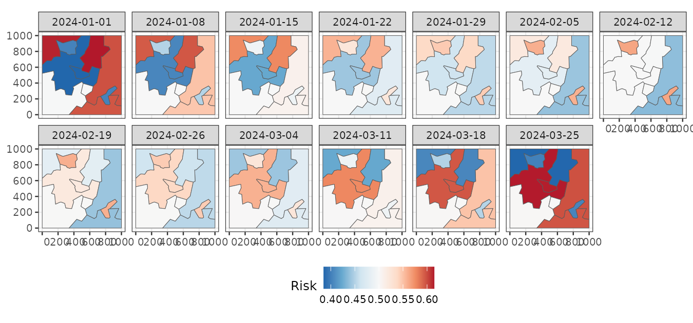

Finally, we can use our clustering results to visualize the original data grouped by clusters using the function plot_clusters_series(). As the output is a ggplot object, then we can easily customize the output as follows:

plot_clusters_series(result, cases/population, sort = TRUE) +
  facet_wrap(~ cluster, ncol = 5)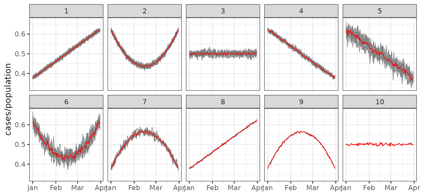

Even though some clusters exhibit similar trends—for example, clusters 2 and 6—the variability between them differs, which justifies their classification as separate clusters.