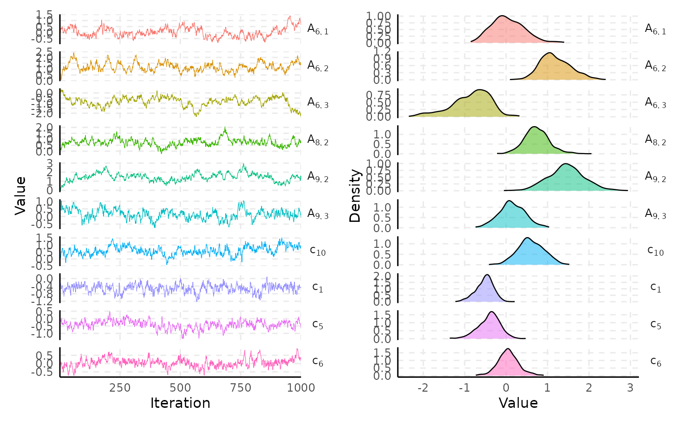
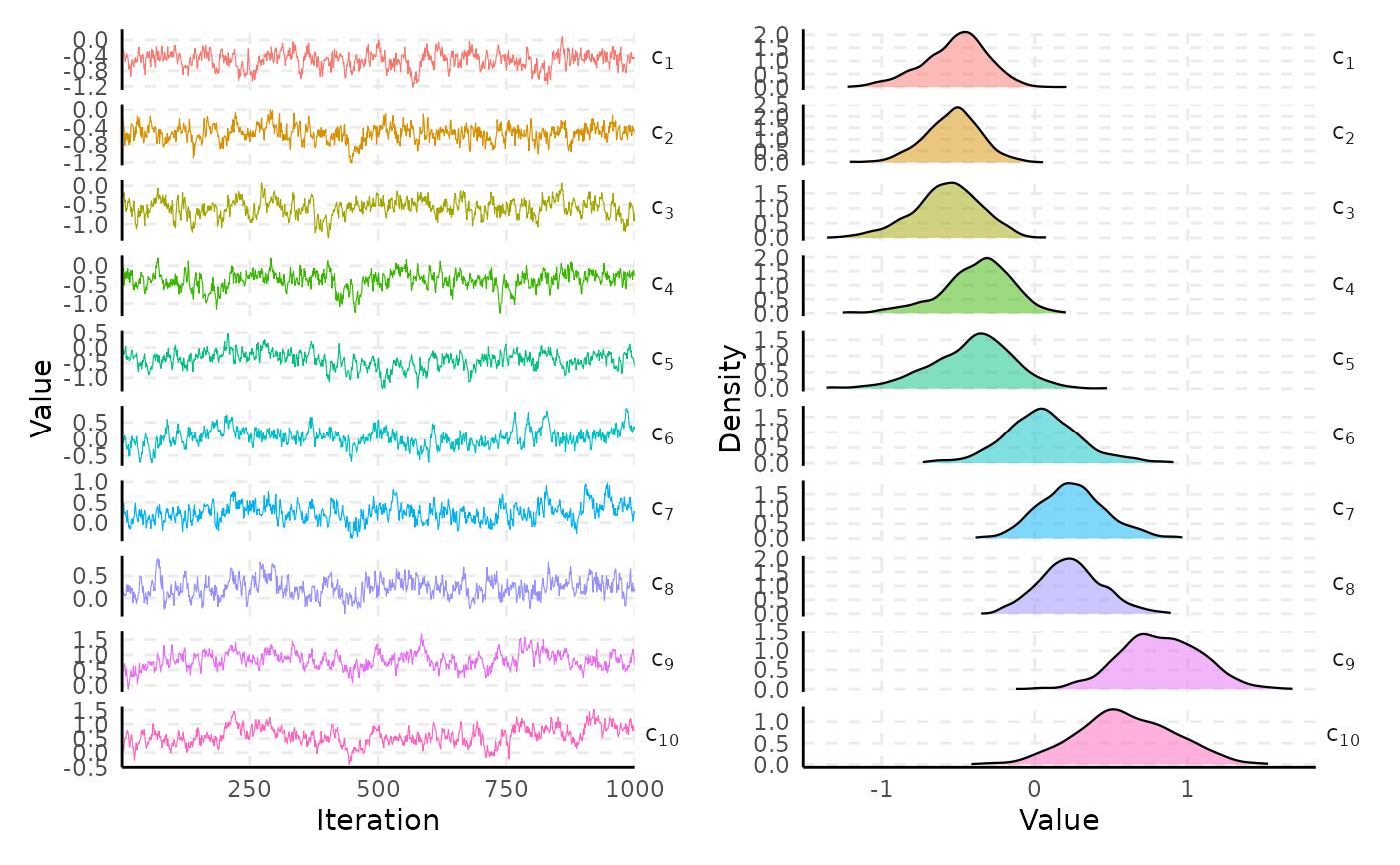
Default Plot of spifa Posterior Samples

The plot default for a fitted spifa object: a combined trace + density view, plot_trace on the left and plot_density on the right, one row per parameter and matched row for row, via wrap_plots – convergence and posterior shape at a glance, right after fitting. Defaults to the easiness (c) and discrimination (A) parameters. For a credible-interval view, or for any other parameter group, call plot_trace/plot_density/ plot_interval directly instead.

Usage

# S3 method for class 'spifa'
plot(x, select = c("c", "A"), nshow = 10, ...)

Arguments

x: A fitted spifa object, as returned by spifa.
select: Parameters to plot, as in plot_trace. Defaults to c("c", "A").
nshow: As in plot_trace, but applied once up front so both panels show the same parameters: calling plot_trace/ plot_density separately with the same select can otherwise each pick a different random subsample.
...: Further arguments passed to both plot_trace and plot_density.

Value

A patchwork object (a ggplot-like object).

Author

Erick A. Chacón-Montalván

Examples

# \donttest{
data(ipixuna)
samples <- spifa(items ~ 1, data = ipixuna, nfactors = 3, ngp = 0, niter = 1000)

plot(samples)

plot(samples, select = "c")

# }